German Credit, step by step

This is one run, start to finish, on a public dataset. Every number on this page came off the platform. Follow along with the same files and you will get something close, though not identical: results vary run to run, and that is explained below.

The problem

Predict whether a credit applicant is a good or bad risk, from the application data. The dataset is the UCI German Credit set: 1,000 applications, 20 features, a binary outcome. It is a well-known benchmark and a genuinely hard one. Only 30% of applicants are bad risks, and that minority is exactly the class you care about. A model that declares everyone good scores 70% accuracy and is worth nothing. The business asymmetry is the usual one. Lending to someone who defaults costs more than declining someone who would have repaid. So recall on the bad class matters more than headline accuracy, and the model you want may not be the one with the fewest errors overall.

The files

Split 80/20, shuffled, labels kept in both.

File	Rows	Columns
german-credit-train.csv	800	id + 20 features + `class`
german-credit-test.csv	200	same, labels kept
german-credit-unlabelled.csv	200	no `class` column

id,checking_status,duration,credit_history,purpose,credit_amount,savings_status,employment,...,class
ca616699-0a9b-44d3-8905-825e23cfca28,0<=X<200,12,critical/other existing credit,new car,2366,...,good

First column is a unique ID, last column is the target with values good and bad.

Part 1: Feature Refinery

Start the run

Feature Refinery → Refine Features.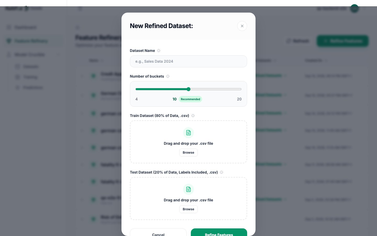

Field	Value
Dataset Name	`German Credit Risk`
Number of buckets	`4`
Train Dataset	`german-credit-train.csv`
Test Dataset	`german-credit-test.csv`

Buckets are set to 4 here because the training file is small, 800 rows. On a larger file, leave it at the recommended 10.

Over the API

# 1. create
curl -s -X POST "$BASE/api/v1/feature-refinery" \
  -H "Authorization: Bearer $TOKEN" -H "Content-Type: application/json" \
  -d '{"name":"German Credit Risk","numberOfBuckets":4,
       "trainFileName":"german-credit-train.csv","testFileName":"german-credit-test.csv"}'
# -> { "featureRefinementKey": "...", "uploadTargets": [ {kind, url, requiredHeader}, ... ] }

# 2. PUT each file to its signed URL (see the API recipes for the headers)
# 3. start
curl -s -X POST "$BASE/api/v1/feature-refinery/$KEY/start" \
  -H "Authorization: Bearer $TOKEN"

Full version in API recipes.

What happens

The run establishes a baseline first: it trains many models on all 21 columns and records how many decisions the best of them got wrong. Then it works through the columns one at a time, removing, retraining, and deciding. Expand the row to watch it. The progress bar and elapsed time are live.

The result

52 minutes.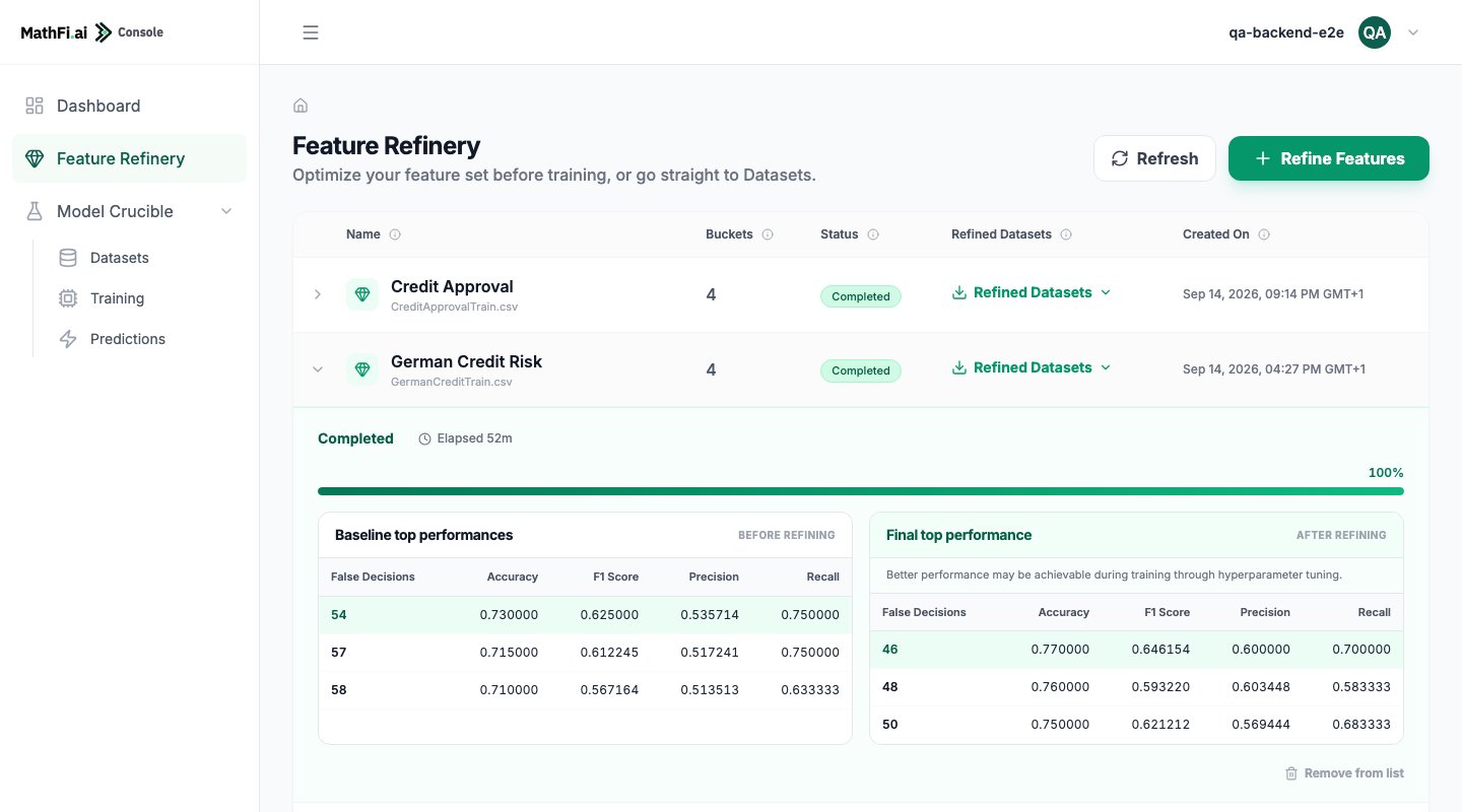

Before refining

54 false decisions · accuracy 0.730 · F1 0.625 · precision 0.536 · recall 0.750

After refining

46 false decisions · accuracy 0.770 · F1 0.646 · precision 0.600 · recall 0.700

Eight fewer wrong decisions out of 200, from removing columns. Nothing was added, no setting was tuned, no model was changed. Columns that were not helping came out. The run also produced the two things the next stage needs:

Column status: one KEEP or REMOVE per original column. Download it from the Refined Datasets menu on the row.
A measured target of roughly 0.70. This is what the refined data can actually reach, and it is the number that makes or breaks the training run.

Run it twice and you will get different numbers. Different baselines, sometimes different column decisions, occasionally a run that removes nothing at all. Many independent trainings are averaged and they do not all land in the same place. Treat one run as evidence, not proof.

Part 2: Model Crucible

Build the dataset

Model Crucible → Datasets → Create Dataset.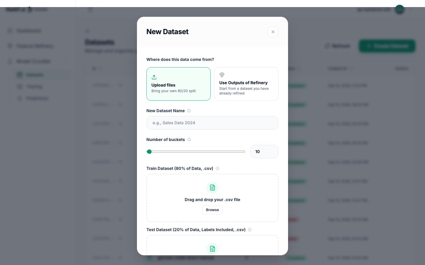

Choose Use Outputs of Refinery and pick German Credit Risk. There is nothing to upload: the refined train and test files come across as they are, already split and already reduced, and the bucket count and measured target come with them. Wait for Completed.

Train

Training → New Training Job.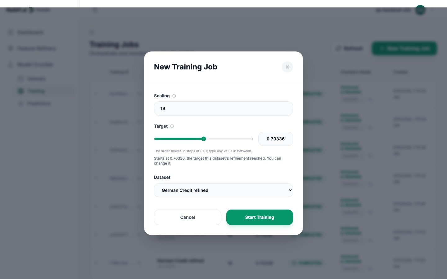

Field	Value
Dataset	`German Credit refined`
Target	`0.70336` (pre-filled from the refinement)
Scaling	`19`

That target is pre-filled because it is the value the refinement reached. Do not raise it because 0.9 sounds better. On this dataset a target of 0.9 gives you a run where every attempt hits its time cap and a champion that labels every applicant good: 70% accuracy, F1 of zero, and a busy grid that looks like it worked.

Over the API

Read the target off the dataset rather than guessing it:

THRESHOLD=$(curl -s -H "Authorization: Bearer $TOKEN" \
  "$BASE/api/v1/datasets/$DATASET_KEY" | jq -r '.recommendedThreshold')

curl -s -X POST "$BASE/api/v1/training/datasets/$DATASET_KEY" \
  -H "Authorization: Bearer $TOKEN" -H "Content-Type: application/json" \
  -d "{\"performanceThreshold\": $THRESHOLD, \"scalingFactor\": 19}"

The result

Minutes, not hours. Open the finished run.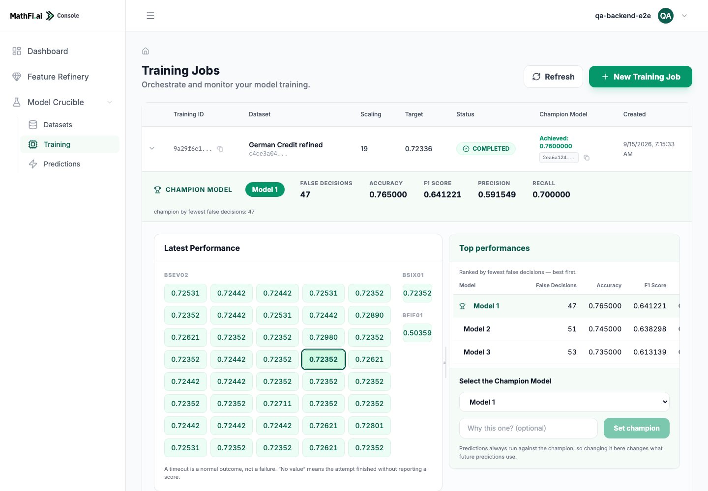

The grid on the left is every attempt, scored live. The table on the right is what the run is offering you:

Model	False decisions	Accuracy	F1	Precision	Recall
Model 1 (champion)	47	0.765	0.641	0.592	0.700
Model 2	51	0.745	0.638
Model 3	53	0.735	0.613

Model 1 is champion by default: fewest wrong decisions.

The refinement’s own scoring pass reported 46 false decisions and this training run landed on 47. That is the same ballpark, and it is what to expect. The refinement’s number tells you what the cleaned data can support. It is not a score the next run inherits.

Choose the champion on your own terms

This is the step people skip, and on this problem it is the step that matters. Model 1 has the fewest errors. That does not automatically make it the model you want. If catching a bad applicant is worth more to you than avoiding an unnecessary decline, then recall on the bad class is what you are buying, and you should take the candidate that gives you more of it even though its total error count is higher. Select it in Select the Champion Model, add a line saying why, and click Set champion. Predictions from that point on run against your choice. Earlier predictions are untouched: each one recorded the version it ran against.

Part 3: Predict

Predictions → New Prediction. Choose the champion model and upload german-credit-unlabelled.csv.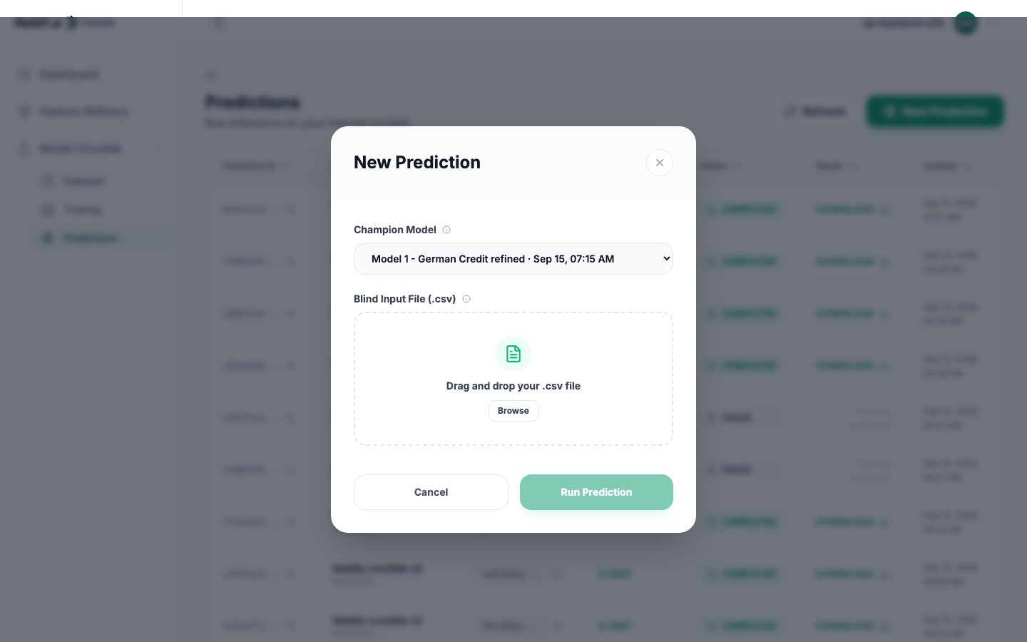

The file has the same columns as the training data, minus class. You do not need to strip the columns the refinement removed; the platform does it for you. When the run completes, download the result: your rows, with the predicted class appended.

Over the API

PRED=$(curl -s -X POST \
  "$BASE/api/v1/predictions?modelKey=$MODEL_KEY&applyColumnStatusFilter=true" \
  -H "Authorization: Bearer $TOKEN" \
  -F "[email protected];type=text/csv" | jq -r '.predictionKey')

# poll until COMPLETED, then follow predictionResultDownloadUrl
curl -s -H "Authorization: Bearer $TOKEN" \
  "$BASE/api/v1/predictions/$PRED" | jq '.status, .predictionResultDownloadUrl'

What the run showed

Stage	False decisions out of 200
All 21 columns, before refining	54
After refining	46
Trained champion	47

The refinement did the work. It took a hard, imbalanced, well-studied dataset and improved it by removing columns, then told the training stage what target to aim for. Training then produced three models to choose between rather than one to accept. Total hands-on time: around ten minutes of clicking. Total wall clock: about an hour, nearly all of it the refinement running unattended. How this compares against tuned XGBoost, LightGBM, CatBoost, Random Forest and Logistic Regression on the same held-back rows is published on the benchmarks page. This run is a separate one from the benchmark, so the figures differ slightly.

The other six use cases

Credit approval, warranty fraud, stroke screening, radar, cardiac disease, mortality risk.

Try it with your own data

The quickstart, without the commentary.

Automate it

The same run driven by a script or an agent.

Input data

Getting your own CSVs into the right shape.

Getting started

Products

Guides

Use cases

German Credit, step by step

The problem

The files

Part 1: Feature Refinery

Start the run

What happens

The result

Before refining

After refining

Part 2: Model Crucible

Build the dataset

Train

The result

Choose the champion on your own terms

Part 3: Predict

What the run showed

The other six use cases

Try it with your own data

Automate it

Input data

​The problem

​The files

​Part 1: Feature Refinery

​Start the run

​What happens

​The result

Before refining

After refining

​Part 2: Model Crucible

​Build the dataset

​Train

​The result

​Choose the champion on your own terms

​Part 3: Predict

​What the run showed

The other six use cases

Try it with your own data

Automate it

Input data

The problem

The files

Part 1: Feature Refinery

Start the run

What happens

The result

Part 2: Model Crucible

Build the dataset

Train

The result

Choose the champion on your own terms

Part 3: Predict

What the run showed